Plasma radiation astronomy
Editor-In-Chief: Henry A. Hoff
A coronal cloud is a cloud, or cloud-like, natural astronomical entity, composed of plasma and usually associated with a star or other astronomical object where the temperature is such that X-rays are emitted. While small coronal clouds are above the photosphere of many different visual spectral type stars, others occupy parts of the interstellar medium (ISM), extending sometimes millions of kilometers into space, or thousands of light-years, depending on the size of the associated object such as a galaxy.
Auroras
{{fairuse}}Auroras can be caused by electrons being absorbed into an atmosphere.
The "dramatic panorama [on the right shows a colorful], shimmering auroral curtain reflected in a placid Icelandic lake. The image was taken on 18 March 2015 by Carlos Gauna, near Jökulsárlón Glacier Lagoon in southern Iceland."[1]
"The celestial display was generated by a coronal mass ejection, or CME, on 15 March. Sweeping across the inner Solar System at some 3 million km per hour, the eruption reached Earth, 150 million kilometres away, in only two days. The gaseous cloud collided with Earth’s magnetic field at around 04:30 GMT on 17 March."[1]
"When the charged particles from the Sun penetrate Earth's magnetic shield, they are channelled downwards along the magnetic field lines until they strike atoms of gas high in the atmosphere. Like a giant fluorescent neon lamp, the interaction with excited oxygen atoms generates a green or, more rarely, red glow in the night sky, while excited nitrogen atoms yield blue and purple colours."[1]
"Auroral displays are not just decorative distractions. They are most frequent when the Sun's activity nears its peak roughly every 11 years. At such times, the inflow of high-energy particles and the buffeting of Earth’s magnetic field may sometimes cause power blackouts, disruption of radio communications, damage to satellites and even threaten astronaut safety."[1]
Coronas
Def. "[t]he luminous plasma atmosphere of the Sun or other star, extending millions of kilometres into space, most easily seen during a total solar eclipse"[2] is called a corona, or stellar corona.
"Beginning with the daguerreotype of the corona of 1851, the Reverend Lecturer had thrown on the screen pictures illustrating the form of the corona in different years. The drawings of those of 1867, 1878, and 1900 all showed long equatorial extensions with openings at the solar poles filled with beautiful rays."[3] "The intermediate years, as, for example, 1883, 1886, and 1896 showed the four groups of synclinals which mainly constitute the corona gradually descending towards the equator of the sun, with a corresponding opening of the polar regions."[3]
"Some of the theories of the solar corona were then illustrated and discussed."[3]
- "The corona is not of the nature of an atmosphere round the sun, for the pressure at the sun's limb would be enormous, while the thinness of the chromospheric lines show that it is not."[3]
- "comets, such as that of 1843, have approached the sun with enormous velocities within the region of the prominences without suffering disruption or retardation."[3]
- "If not an atmosphere of particles of gas, still less is it an atmosphere of solid stones or meteorites."[3]
- "Meteor streams do circle round the sun, but there is no reason why the positions of the orbits, or the intrinsic brightness of such streams should vary with the sun-spot period."[3]
- "the appearance of the corona does not seem to be such as the projection of meteor streams upon the celestial vault would give."[3]
- "Prof. Schaeberle has proposed a mechanical origin of the solar corona, due to the forces of ejection of particles from the solar limb, as evidenced by the prominences, and the force of gravity under the particular conditions of the solar rotation and the inclination of its axis to the earth's orbit."[3]
- "The electrical theory of the corona does not negative the mechanical theory, but supplements it. In addition to the forces of gravity and ejection, it takes account of the repulsive force which the sun exerts on matter which has the same electrical sign as itself, and which has been ejected from it."[3]
- "it would seem that the solar corona is of the nature of an electrical aurora round the sun."[3]
- "the coronoidal discharges in poor vacua obtained by Prof. Pupin about an insulated metal ball are exceedingly like the rays and streamers of the solar corona."[3]
The Sun's hot corona continuously expands in space creating the solar wind, a stream of charged particles that extends to the heliopause at roughly 100 astronomical units. The bubble in the interstellar medium formed by the solar wind, the heliosphere, is the largest continuous structure in the Solar System.[4][5]
The sun's corona is constantly being lost to space, creating what is essentially a very thin atmosphere throughout the Solar System. The movement of mass ejected from the Sun is known as the solar wind. Inconsistencies in this wind and larger events on the surface of the star, such as coronal mass ejections, form a system that has features analogous to conventional weather systems (such as pressure and wind) and is generally known as space weather. Coronal mass ejections have been tracked as far out in the solar system as Saturn.[6] The activity of this system can affect planetary atmospheres and occasionally surfaces. The interaction of the solar wind with the terrestrial atmosphere can produce spectacular aurorae,[7] and can play havoc with electrically sensitive systems such as electricity grids and radio signals.
Coronal arcades
Def. a close collection of loops in a cylindrical structure is called an arcade.
The TRACE image at right "is from near flare maximum (11:00 UT) and has a width of 230,000 km [...] how in the world can the footpoints of the arcade have such a clearly-organized pattern whose scale greatly exceeds the known scales of the largest convective scales known in the photosphere?"[8]
"The most obvious coronal signatures of CMEs in the low corona are the arcades of bright loops that develop after the CME material has erupted [...] nearly all (92%) EIT post-eruptive arcades from 1997 – 2002 were associated with LASCO CMEs [...] The activity associated with halo CMEs includes the formation of dimming regions, long-lived loop arcades, flaring active regions, large-scale coronal waves and filament eruptions".[9]
Coronal clouds
"Coronal clouds, type IIIg, form in space above a spot area and rain streamers upon it."[10]
"[C]oronal magnetic bottles, produced by flares, [may] serve as temporary traps for solar cosmic rays ... It is the expansion of these bottles at velocities of 300–500 km/s which allows fast azimuthal propagation of solar cosmic rays independent of energy. A coronagraph on Os 7 observed a coronal cloud which was associated with bifurcation of the underlying coronal structure."[11]
In a coronal cloud are magnetohydrodynamic plasma flux tubes along magnetic field lines.[12]
Coronal heating
"The photosphere of the Sun has an effective temperature of 5,570 K[13] yet its corona has an average temperature of 1–2 x 10⁶ K.[14] However, the hottest regions are 8–20 x 106 K.[14] The high temperature of the corona shows that it is heated by something other than direct heat conduction from the photosphere.[15]
It is thought that the energy necessary to heat the corona is provided by turbulent motion in the convection zone below the photosphere, and two main mechanisms have been proposed to explain coronal heating.[14] The first is wave heating, in which sound, gravitational or magnetohydrodynamic waves are produced by turbulence in the convection zone.[14] These waves travel upward and dissipate in the corona, depositing their energy in the ambient gas in the form of heat.[16] The other is magnetic heating, in which magnetic energy is continuously built up by photospheric motion and released through magnetic reconnection in the form of large solar flares and myriad similar but smaller events—nanoflares.[17]
Currently, it is unclear whether waves are an efficient heating mechanism. All waves except Alfvén waves have been found to dissipate or refract before reaching the corona.[18] In addition, Alfvén waves do not easily dissipate in the corona. Current research focus has therefore shifted towards flare heating mechanisms.[14]"[19]
Coronal loops
Coronal loops have become very important when trying to understand the current coronal heating problem. Coronal loops are highly radiating sources of plasma and therefore easy to observe by instruments such as TRACE; they are highly observable laboratories to study phenomena such as solar oscillations, wave activity and nanoflares. However, it remains difficult to find a solution to the coronal heating problem as these structures are being observed remotely, where many ambiguities are present (i.e. radiation contributions along the [line-of-sight propagation] LOS). In-situ measurements are required before a definitive answer can be arrived at, but due to the high plasma temperatures in the corona, in-situ measurements are impossible (at least for the time being). The next mission of the Nasa Solar Probe Plus will approach the Sun very closely allowing more direct observations.
"The peak continuum intensity was always at the loop tops."[20]
The population of coronal loops can be directly linked with the solar cycle; it is for this reason coronal loops are often found with sunspots at their footpoints. Coronal loops project through the chromosphere and transition region, extending high into the corona.
Coronal loops have a wide variety of temperatures along their lengths. Loops existing at temperatures below 1 MK are generally known as cool loops, those existing at around 1 MK are known as warm loops, and those beyond 1 MK are known as hot loops. Naturally, these different categories radiate at different wavelengths.[21]
Coronal loops populate both active and quiet regions of the solar surface. Active regions on the solar surface take up small areas but produce the majority of activity and 82% of the total coronal heating energy.[12] The quiet Sun, although less active than active regions, is awash with dynamic processes and transient events (bright points, nanoflares and jets).[22] As a general rule, the quiet Sun exists in regions of closed magnetic structures, and active regions are highly dynamic sources of explosive events. It is important to note that observations suggest the whole corona is massively populated by open and closed magnetic fieldlines. A closed fieldline does not constitute a coronal loop; however, closed flux must be filled with plasma before it can be called a coronal loop.
The image at right shows particle rays leaving the surface of the Sun (darker ends of the loops), traveling in a loop controlled by a local magnetic field similar to how particle accelerators accelerate, steer, and aim a stream of particles at a target (the much brighter regions in the chromosphere). The loops have a temperature of approximately 106 K and are emitting X-rays (synchrotron and cyclotron radiation).
Coronal loops form the basic structure of the lower corona andtransition region of the Sun. These highly structured and elegant loops are a direct consequence of the twisted solar magnetic flux within the solar body. The population of coronal loops can be directly linked with the solar cycle; it is for this reason coronal loops are often found with sunspots at their footpoints. The upwelling magnetic flux pushes through the photosphere, exposing the cooler plasma below.
Loops of magnetic flux (closed flux tubes) well up from the solar body and fill with hot solar plasma.[23] Due to the heightened magnetic activity in these coronal loop regions, coronal loops can often be the precursor to solar flares and coronal mass ejections (CMEs).
Coronal mass ejections
Def. a "massive burst of solar wind, other light isotope plasma, and magnetic fields rising above the solar corona or being released into space"[24] is called a coronal mass ejection (CME).
An explosive limb flare occurred above 30,000 km in the corona of the Sun.[25] "So the aftermath of the flare explosion, usually visible in disk pictures as extensive Hα brightening, but hidden from us in this case, was seen by the ionosphere as an intense flux of ionizing radiation from the coronal cloud created by the explosion."[25] "The November 20, 1960, event is very similar to that of February 10, 1956, which was observed at Sacramento Peak. A bright ball appears above the surface, grows in size and Hα brightness, and explodes upward and outward."[25] "The great breadth and intensity of the Hα emission from the suspended ball at 2013 U.T. testify to the large amount of energy stored there, as no corresponding macroscopic motion was observed until the explosion at 2023 U.T."[25] "[T]he great energy of the preflare cloud was released into the corona by the explosion of 2023 U.T., and Hα radiation disappeared by 2035 U.T."[25]
"On 16 June 1972, the Naval Research Laboratory's coronagraph aboard OSO-7 tracked a huge coronal cloud moving outward from the Sun."[26]
A coronal mass ejection (CME) is an ejected plasma consisting primarily of electrons and protons (in addition to small quantities of heavier elements such as helium, oxygen, and iron), plus the entraining coronal closed magnetic field regions. Evolution of these closed magnetic structures in response to various photospheric motions over different time scales (convection, differential rotation, meridional circulation) somehow leads to the CME.[27] Small-scale energetic signatures such as plasma heating (observed as compact soft X-ray brightening) may be indicative of impending CMEs.
The soft X-ray sigmoid (an S-shaped intensity of soft X-rays) is an observational manifestation of the connection between coronal structure and CME production.[27]
"Relating the sigmoids at X-ray (and other) wavelengths to magnetic structures and current systems in the solar atmosphere is the key to understanding their relationship to CMEs."[27]
Coronal streamers
The interconnections of active regions are arcs connecting zones of opposite magnetic field, in different active regions. Significant variations of these structures are often seen after a flare. Some other features of this kind are helmet streamers—large cap-like coronal structures with long pointed peaks that usually overlie sunspots and active regions. Coronal streamers are considered as sources of the slow solar wind.[28]
Dynamos
"A plasma with local magnetohydrodynamic instabilities creates mechanical turbulence, motion, or shear (a dynamo) which in turn generates or sustains the local magnetic field."[29]
Electromagnetics
"The first systematic attempt to base a theory of the origin of the solar system on electromagnetic or hydromagnetic effects was made in Alfvén (1942). The reason for doing so was that a basic difficulty with the old Laplacian hypothesis: how can a central body (Sun or planet) transfer angular momentum to the secondary bodies (planets or satellites) orbiting around it? It was demonstrated that this could be done by electromagnetic effects. No other acceptable mechanism has yet been worked out. [...] the electromagnetic transfer mechanism has been confirmed by observations, as described in the monograph Cosmic Plasma (Alfvén, 1981, pp. 28, 52, 53 0."[30]
"If charged particles (electrons, ions or charged grains) move in a magnetic dipole field - strong enough to dominate their motion - under the action of gravitation and the centrifugal force, they will find an equilibrium in a circular orbit if their centrifugal force is 2/3 of the gravitational force [...] The consequence of this is that if they become neutralized, so that electromagnetic forces disappear, the centrifugal force is too small to balance the gravitation. Their circular orbit changes to an elliptical orbit with the semi-major axis a = 3/4a0 and e = 1/3 (where a0 is the central distance where the neutralization takes place [...] Collisional (viscous) interaction between the condensed particles will eventually change the orbit into a new circular orbit with a = 2/3a0 and e = 0."[30]
"If [...] there is plasma in the region [collisional interaction results in] matter in the 2/3-[region]. [...] matter in the region [...] will produce a [cosmogonic] shadow in the region".[30]
Electron winds
As of December 5, 2011, "Voyager 1 is about ... 18 billion kilometers ... from the [S]un [but] the direction of the magnetic field lines has not changed, indicating Voyager is still within the heliosphere ... the outward speed of the solar wind had diminished to zero in April 2010 ... inward pressure from interstellar space is compacting [the magnetic field] ... Voyager has detected a 100-fold increase in the intensity of high-energy electrons from elsewhere in the galaxy diffusing into our solar system from outside ... [while] the [solar] wind even blows back at us."[31]
Flares
"[A] medium-strength flare erupted from the sun on July 19, 2012. The blast also generated the enormous, shimmering plasma loops, which are an example of a phenomenon known as "coronal rain," agency officials said."[32]
"The ... solar proton flare on 20 April 1998 at W 90° and S 43° (9:38 UT) was measured by the GOES-9-satellite (Solar Geophysical Data 1998), as well as by other experiments on WIND ... and GEOTAIL. Protons were accelerated up to energies > 110 MeV and are therefore able to hit the surface of Mercury."[33]
Flare stars
"Flare stars are intrinsically faint, but have been found to distances of 1,000 light years from Earth.[34]
Galactic coronas
Although a galactic corona is usually "filled with high-temperature plasma at temperatures of T ≈ 1–2 (MK), ... [h]ot active regions and postflare loops have plasma temperatures of T ≈ 2–40 MK."[35]
"Discussion of the alternative hypothesis of cloud ejection from the equatorial layer of the Galaxy leads to the conclusion that the gaseous halo must be highly turbulent and that the coronal clouds are probably H I regions".[36]
"One question posed by these previous observations is where the absorption originates. If a coronal cloud, the cloud is more than 15 kpc from the plane of NGC 3067. This distance is greater than the optical radius of the galaxy, 9.6 kpc (H = 50 km s-1 Mpc-1. Furthermore, the narrow line requires that the cloud be cool, in contrast to the wide range of ionization stages detected for the corona of our Galaxy (Savage and deBoer 1981)."[37] "But if the cloud originates instead in the disk, and is moving in a circular orbit viewed at an inclination of 68 deg (the inclination of the optical galaxy), then some gas extends at least to 40 kpc, which is over four times the optical radius."[37]
Helmet streamers
Helmet streamers are bright loop-like structures which develop over active regions on the sun. They are closed magnetic loops which connect regions of opposite magnetic polarity. Electrons are captured in these loops, and cause them to glow very brightly. The solar wind elongates these loops to pointy tips. They far extend above most prominences into the corona, and can be readily observed during a solar eclipse. Helmet streamers are usually confined to the "streamer belt" in the mid latitudes, and their distribution follows the movement of active regions during the solar cycle. Small blobs of plasma, or "plasmoids" are sometimes released from the tips of helmet streamers, and this is one source of the slow component of the solar wind. In contrast, formations with open magnetic field lines are called coronal holes, and these are darker and are a source of the fast solar wind. Helmet streamers can also create coronal mass ejections if a large volume of plasma becomes disconnected near the tip of the streamer.
Ionospheres
Upon reaching the top of the mesosphere, the temperature starts to rise, but air pressure continues to fall. This is the beginning of the ionosphere, a region dominated by chemical ions. Many of them are the same chemicals such as nitrogen and oxygen in the atmosphere below, but an ever increasing number are hydrogen ions (protons) and helium ions. These can be detected by an ion spectrometer. The process of ionization removes one or more electrons from a neutral atom to yield a variety of ions depending on the chemical element species and incidence of sufficient energy to remove the electrons.
Def. the "part of the Earth's atmosphere beginning at an altitude of about 50 kilometers [31 miles] and extending outward 500 kilometers [310 miles] or more"[38] or the "similar region of the atmosphere of another planet"[39] is called an ionosphere.
"As a spacecraft travels through the solar system, a targeted radio signal sent back to Earth can be aimed through the ionosphere of a nearby planet. Plasma in the ionosphere causes small but detectable changes in the signal that allow scientists to learn about the upper atmosphere."[40]
Io plasma torus
The image at right represents "[t]he Jovian magnetosphere [magnetic field lines in blue], including the Io flux tube [in green], Jovian aurorae, the sodium cloud [in yellow], and sulfur torus [in red]."[41]
"Io may be considered to be a unipolar generator which develops an emf [electromotive force] of 7 x 10⁵ volts across its radial diameter (as seen from a coordinate frame fixed to Jupiter)."[42]
"This voltage difference is transmitted along the magnetic flux tube which passes through Io. ... The current [in the flux tube] must be carried by keV electrons which are electrostatically accelerated at Io and at the top of Jupiter's ionosphere."[42]
"Io's high density (4.1 g cm-3) suggests a silicate composition. A reasonable guess for its electrical conductivity might be the conductivity of the Earth's upper mantle, 5 x 10⁻⁵ ohm-1 cm-1 (Bullard 1967)."[42]
As "a conducting body [transverses] a magnetic field [it] produces an induced electric field. ... The Jupiter-Io system ... operates as a unipolar inductor" ... Such unipolar inductors may be driven by electrical power, develop hotspots, and the "source of heating [may be] sufficient to account for the observed X-ray luminosity".[43]
"The electrical surroundings of Io provide another energy source which has been estimated to be comparable with that of the [gravitational] tides (7). A current of 5 x 10⁶ A is ... shunted across flux tubes of the Jovian field by the presence of Io (7-9)."[44]
"[W]hen the currents [through Io] are large enough to cause ohmic heating ... currents ... contract down to narrow paths which can be kept hot, and along which the conductivity is high. Tidal heating [ensures] that the interior of Io has a very low eletrical resistance, causing a negligible extra amount of heat to be deposited by this current. ... [T]he outermost layers, kept cool by radiation into space [present] a large resistance and [result in] a concentration of the current into hotspots ... rock resistivity [and] contact resistance ... contribute to generate high temperatures on the surface. [These are the] conditions of electric arcs [that can produce] temperatures up to ionization levels ... several thousand kelvins".[44]
"[T]he outbursts ... seen [on the surface may also be] the result of the large current ... flowing in and out of the domain of Io ... Most current spots are likely to be volcanic calderas, either provided by tectonic events within Io or generated by the current heating itself. ... [A]s in any electric arc, very high temperatures are generated, and the locally evaporated materials ... are ... turned into gas hot enough to expand at a speed of 1 km/s."[44]
Local hot bubbles
The 'local hot bubble' is a "hot X-ray emitting plasma within the local environment of the Sun."[45] "This coronal gas fills the irregularly shaped local void of matter (McCammon & Sanders 1990) - frequently called the Local Hot Bubble (LHB)."[45]
"The [X-ray] intensity of the [Local Hot Bubble] LHB varies across the entire sky:"[46]
- ILHB = (2.5-8.2) x 10-4 cts s-1 arcmin-2 (Snowden et al. 1998).
The galactic X-ray background is produced largely by emission from the Local Hot Bubble which is within 100 parsecs of the Sun. The Local Hot Bubble is within the Local Bubble.
Magnetic clouds
A magnetic cloud is a transient event observed in the solar wind. It was defined in 1981 by Burlaga et al. 1981 as a region of enhanced magnetic field strength, smooth rotation of the magnetic field vector and low proton temperature [47]. Magnetic clouds are a possible manifestation of a Coronal Mass Ejection (CME). The association between CMEs and magnetic clouds was made by Burlaga et al. in 1982 when a magnetic cloud was observed by Helios-1 two days after being observed by SMM[48]. However, because observations near Earth are usually done by a single spacecraft, many CMEs are not seen as being associated with magnetic clouds. The typical structure observed for a fast CME by a satellite such as ACE is a fast-mode shock wave followed by a dense (and hot) sheath of plasma (the downstream region of the shock) and a magnetic cloud.
Other signatures of magnetic clouds are now used in addition to the one described above: among other, bidirectional superthermal electrons, unusual charge state or abundance of iron, helium, carbon and/or oxygen. The typical time for a magnetic cloud to move past a satellite at the L1 point is 1 day corresponding to a radius of 0.15 AU with a typical speed of 450 km s−1 and magnetic field strength of 20 nT [49]
Magnetic reconnections
Magnetic reconnection is a physical process in highly conducting plasmas in which the magnetic topology is rearranged and magnetic energy is converted to kinetic energy, thermal energy, and particle acceleration. Magnetic reconnection occurs on timescales intermediate between slow resistive diffusion of the magnetic field and fast Alfvénic timescales. The qualitative description of the reconnection process is such that magnetic field lines from different magnetic domains (defined by the field line connectivity) are spliced to one another, changing their patterns of connectivity with respect to the sources. It is a violation of an approximate conservation law in plasma physics, and can concentrate mechanical or magnetic energy in both space and time.
Magnetospheres
A magnetosphere is formed when a stream of charged particles, such as the solar wind, interacts with and is deflected by the magnetic field of a planet or similar body.
“Planets which generate magnetic fields in their interiors ... are surrounded by invisible magnetospheres. ... [I]n many respects, the magnetosphere of Venus is a scaled-down version of Earth’s. ... Earth’s magnetosphere is 10 times larger [than that of Venus]”[50]
Microflares
Ultraviolet telescopes such as TRACE and SOHO/EIT can observe individual [solar] micro-flares as small brightenings in extreme ultraviolet light.[51]
Nanoflares
The image at the right shows the first detection of high temperature nanoflares. The false-color temperature map of solar active region AR10923, observed close to center of the sun's disk, contains nanoflare regions (blue, indicating plasma near 10 million degrees K).
"Nanoflares are small, sudden bursts of heat and energy. "They occur within tiny strands that are bundled together to form a magnetic tube called a coronal loop," says Klimchuk. Coronal loops are the fundamental building blocks of the thin, translucent gas known as the sun's corona. ... Observations from the NASA-funded X-Ray Telescope (XRT) and Extreme-ultraviolet Imaging Spectrometer (EIS) instruments aboard Hinode reveal that ultra-hot plasma is widespread in solar active regions. The XRT measured plasma at 10 million degrees K, and the EIS measured plasma at 5 million degrees K. "These temperatures can only be produced by impulsive energy bursts,"says Klimchuk ... "Coronal loops are bundles of unresolved strands that are heated by storms of nanoflares." ... when a nanoflare suddenly releases its energy, the plasma in the low-temperature, low-density strands becomes very hot—around 10 million degrees K—very quickly. The density remains low, however, so the emission, or brightness, remains faint. Heat flows from up in the strand, where it's hot, down to the base of the coronal loop, where it's not as hot. This heats up the dense plasma at the loop’s base. Because it is so dense at the base, the temperature only reaches about 1 million degrees K. This dense plasma expands up into the strand. Thus, a coronal loop is a collection of 5-10 million degree K faint strands and 1 million degree K bright strands. "What we see is 1 million degree K plasma that has received its energy from the heat flowing down from the superhot plasma," says Klimchuk. "For the first time, we have detected this 10 million degree plasma, which can only be produced by the impulsive energy bursts of nanoflares.""[52]
The idea that nanoflares might heat the corona was put forward by Eugene Parker in the 1980s but is still controversial. In particular, ultraviolet telescopes such as TRACE and SOHO/EIT can observe individual micro-flares as small brightenings in extreme ultraviolet light,[51] but there seem to be too few of these small events to account for the energy released into the corona. The additional energy not accounted for could be made up by wave energy, or by gradual magnetic reconnection that releases energy more smoothly than micro-flares and therefore doesn't appear well in the TRACE data. Variations on the micro-flare hypothesis use other mechanisms to stress the magnetic field or to release the energy, and are a subject of active research in 2005.
A nanoflare is a very small solar flare which happens in the corona, the external atmosphere of the Sun. Observations show that the solar magnetic field, which is frozen into the motion of the plasma opens into semicirculal structures in the corona. These coronal loops, which can be seen in the EUV and X-ray images (see the figure on the left), confine very hot plasma, emitting as it were at a temperature of a few million degrees. Many flux tubes are stable for several days on the solar corona in the X-ray images, emitting at steady rate. However flickerings, brightenings, small explosions, bright points, flares and mass eruptions are observed very frequently, especially in active regions. These macroscopic signs of solar activity are considered by astrophysicists as the phenomenology related to events of relaxation of stressed magnetic fields, during which part of the coronal heating is released by current dissipation or Joule effect. These nanoflares might be very tiny flares, so close one to each other, both in time and in space, to heat the corona and to cause all the phenomena due to solar activity.
The distribution of the number of flares observed in the hard X-rays is a function of the energy, following a power law with negative spectral index 1.8.[53][54][55] [56] If this distribution would have the same spectral index also at lower energies, flares, micro-flares and nanoflares might provide a considerable part of coronal heating. Actually a negative spectral index of the order of 2 is required in order to maintain the solar corona.
"[T]he importance of the magnetic field is recognized by all the scientists: there is a strict correspondence between the active regions, where the irradiated flux is higher (especially in the X-rays), and the regions of intense magnetic field.[57]
More energy is released in turbulent regimes when nanoflares happen at much smaller scale-lengths, where non-linear effects are not negligible.[58]
In order to heat a region of very high X-ray emission, over an area 1" x 1", a nanoflare of 1017 J should happen every 20 seconds, and 1000 nanoflares per second should occur in a large active region of 105 x 105 km2.
Flickerings, brightenings, small explosions, bright points, flares and mass eruptions are observed very frequently, especially in active regions.
Nova-like stars
The evolution of non-magnetic dwarf novae and nova-like stars can be different from the magnetic systems (polars and intermediate polars).[59] Magnetic and non-magnetic systems display different kinematical properties since some flow velocities come from magnetically channeled plasma.[59]
Photospheres
The solar photosphere is a "weakly ionized [ni/(ni + na)] ~ 10-4, relatively cold and dense plasma".[60]
Plages
A plage is a bright region in the chromosphere of [a star], typically found in regions of the chromosphere near [starspots]. The plage regions map closely to the faculae in the photosphere below, but the latter have much smaller spatial scales. Accordingly plage occurs most visibly near a starspot region.
"Plages are formed in the inner parts of flux loops emerging from below. ... In the early stages of active region growth the appearance of the group is symmetric, while a few days later the f spot may disappear, leaving an extensive plage."[61]
"[M]ajor changes in active regions only take place in the following ways:
- [starspot] formation and break up;
- flux outflow from [starspots];
- new flux emergence; and
- magnetic reconnection."[61]
"In general there is no proper motion at all in the plage or the surrounding plagettes except for the latter two."[61]
Plasma objects
Plasma is a state of matter similar to gas in which a certain portion of the particles are ionized. Heating a gas may ionize its molecules or atoms (reduce or increase the number of electrons in them), thus turning it into a plasma, which contains charged particles: positive ions and negative electrons or ions.[62]
For plasma to exist, ionization is necessary. The term "plasma density" by itself usually refers to the "electron density", that is, the number of free electrons per unit volume. The degree of ionization of a plasma is the proportion of atoms that have lost or gained electrons, and is controlled mostly by the temperature. Even a partially ionized gas in which as little as 1% of the particles are ionized can have the characteristics of a plasma (i.e., response to magnetic fields and high electrical conductivity). The degree of ionization, α is defined as α = ni/(ni + na) where ni is the number density of ions and na is the number density of neutral atoms. The electron density is related to this by the average charge state <Z> of the ions through ne = <Z> ni where ne is the number density of electrons.
"Plasma is the fourth state of matter, consisting of electrons, ions and neutral atoms, usually at temperatures above 104 degrees Kelvin."[63] "The sun and stars are plasmas; the earth's ionosphere, Van Allen belts, magnetosphere, etc., are all plasmas. Indeed, plasma makes up much of the known matter in the universe."[63]
Plasma rains
"Hot plasma in the corona cooled and condensed along strong magnetic fields in the region" slowly falling back to the solar surface as plasma "rain".[32]
Prominences
A prominence is a large, bright feature extending outward from [a star's] surface, often in a loop shape. Prominences are anchored to [a star's] surface in the photosphere, and extend outwards into the [star's] corona. While the corona consists of extremely hot ionized gases, known as plasma, which [does] not emit much visible light, prominences contain much cooler plasma, similar in composition to that of the chromosphere. A prominence forms over timescales of about a day, and stable prominences may persist in the corona for several months. Some prominences break apart and give rise to coronal mass ejections.
A typical prominence extends over many thousands of kilometers; the largest on record was estimated at over 800,000 kilometres (500,000 mi) long[64] – roughly the radius of the Sun.
"When a prominence is viewed from a different perspective so that it is against the [star] instead of against space, it appears darker than the surrounding background. This formation is instead called a [stellar] filament.[64] It is possible for a projection to be both a filament and a prominence. Some prominences are so powerful that they throw out matter from the [star] into space at speeds ranging from 600 km/s to more than 1000 km/s. Other prominences form huge loops or arching columns of glowing gases over [starspots] that can reach heights of hundreds of thousands of kilometres. Prominences may last for a few days or even for a few months.[65] Flocculi (plural of flocculus) is another term for these filaments, and dark flocculi typically describes the appearance of [stellar] prominences when viewed against the [stellar] disk in certain wavelengths.
Regions
The preflare solar material is observed "to be an elevated cloud of prominence-like material which is suddenly lit up by the onslaught of hard electrons accelerated in the flare; the acceleration may be inside or outside the cloud, and brightening is seen in other areas of the solar surface on the same magnetic field lines."[66]
"A hot coronal cloud at T ~ 107 K is left behind, presumably evaporated from the original material."[66] "[O]nce ionized, the gas is rapidly heated by Coulomb collisions to the coronal cloud temperature, but as this material peels off, a cooler hydrogen-emitting region is left."[66]
Regions which are not in coronal holes are "called 'coronal cloud' regions after their appearance in photographs of the Sun taken in soft X-rays, which most dramatically show up coronal holes."[67] These 'coronal cloud' regions are "in fact the majority of the solar surface."[67]
Lying at a level above the 104 K isotherm, "the thermally conducted flux is negligible, and bounded by the magnetic surfaces between open field (coronal hole) and closed field (coronal cloud) regions."[67] "[C]oronal cloud regions produce no solar wind," but "[s]ome of the input energy may pass out of the cloud regions into the region where the wind is accelerated, thereby contributing to this process."[67]
In the image at right the iron (Fe XIV) green line is followed by doppler imaging to show associated relative coronal plasma velocity towards (-7 km/s side) and away from (+7 km/s side) the large angle spectrometric coronagraph LASCO satellite camera.
Starquakes
"The phenomenon of flare induced sunquakes - waves in the photosphere - discovered by Kosovichev and Zharkova (1998) and now widely studied (e.g. Kosovichev 2006) should also result from the momentum impulse delivered by a cometary impact."[68]
A Moreton wave is the chromospheric signature of a large-scale solar coronal shock wave. Described as a kind of solar 'tsunami',[69] they are generated by solar flares[70][71][72].
The 1995 launch of the Solar and Heliospheric Observatory led to observation of coronal waves, which cause Moreton waves. (SOHO's EIT instrument discovered another, different wave type called 'EIT waves'.)[73] The reality of Moreton waves (aka fast-mode MHD waves) has also been confirmed by the two STEREO spacecraft. They observed a 100,000-km-high wave of hot plasma and magnetism, moving at 250 km/second, in conjunction with a big coronal mass ejection in February 2009.[74][75]
Moreton waves propagate at a speed of usually 500–1500 km/s. Yutaka Uchida interpreted Moreton waves as MHD fast mode shock waves propagating in the corona.[76] He links them to type II radio bursts, which are radio wave discharges created when coronal mass ejections accelerate shocks.[77]
Moreton waves can be observed primarily in the Hα band.[78]
Stellar cycles
The solar cycle has a great influence on space weather, and a significant influence on the Earth's climate since the Sun's luminosity has a direct relationship with magnetic activity.[79] Solar activity minima tend to be correlated with colder temperatures, and longer than average solar cycles tend to be correlated with hotter temperatures. In the 17th century, the solar cycle appeared to have stopped entirely for several decades; few sunspots were observed during this period. During this era, known as the Maunder minimum or Little Ice Age, Europe experienced unusually cold temperatures.[80] Earlier extended minima have been discovered through analysis of tree rings and appear to have coincided with lower-than-average global temperatures.[81]
"MOST current literature on solar activity assumes that the planets do not affect it, and that conditions internal to the Sun are primarily responsible for the solar cycle. Bigg1, however, has shown that the period of Mercury's orbit appears in the sunspot data, and that the influence of Mercury depends on the phases of Venus, Earth, and Jupiter."[82]
"It is shown that starting with the alignment of Venus with Jupiter at perihelion position, these two planets will perfectly align at Jupiter's perihelion after every 23.7 years".[83]
"The tidal forces hypothesis for solar cycles has been proposed by Wood (1972) and others. Table 2 below shows the relative tidal forces of the planets on the sun. Jupiter, Venus, Earth and Mercury are called the "tidal planets" because they are the most significant. According to Wood, the especially good alignments of J-V-E with the sun which occur about every 11 years are the cause of the sunspot cycle. He has shown that the sunspot cycle is synchronous with the alignments, and J. Schove's data for 1500 year of sunspot maxima supports the 11.07 year J-V-E period average."[84]
"Both the 11.86 year Jupiter tropical period (time between perihelion's or closest approaches to the sun and the 9.93 year J-S alignment periods are found in sunspot spectral analysis. Unfortunately direct calculations of the tidal forces of all planets does not support the occurrence of the dominant 11.07 year cycle. Instead, the 11.86 year period of Jupiter's perihelion dominates the results. This has caused problems for several researchers in this field."[84]
"[B]y assuming a harmonic variation having a period of 11.13 years ... the phases of such a variation [in polar diameter minus equatorial diameter of the Sun] coincide to within one-fifth of a year with the phases of the sun-spot fluctuations; that, at times corresponding to minimum of sun-spottedness, the polar diameter is relatively larger; that, at times of maximum sun-spottedness, the equatorial diameter is relatively larger. The amplitude of the variation is extremely small, but its reality would seem to be established. [This] at least renders the existence of such periodic fluctuations in the shape of the sun more probable than their non-existence."[85]
"Solar oblateness, the difference between the equatorial and polar diameters, reflects certain fundamental properties of the Sun. ... the oblateness reflects properties of the Sun's interior, ... [There is] a time varying, excess equatorial brightness [producing] a difference between the equatorial and polar limb darkening functions ... at times when the excess brightness is reduced, the intrinsic visual oblateness can be obtained from the observations without detailed knowledge of the excess brightness. A period of reduced excess brightness occurred in 1973 September."[86] The period of reduced excess equatorial brightness occurred between solar cycle maximum around 1970 and minimum around 1975. Considering excess equatorial brightness and seeking to perform measurements at opportunities of reduced excess equatorial brightness has the effect of reducing solar oblateness from some 86.6 ± 6.6 milli-arcsec to 18.4 ± 12.5 milli-arcsec.[86]
The Babcock Model describes a mechanism which can explain magnetic and sunspot patterns observed on the Sun:
- The start of the 22-year cycle begins with a well-established dipole field component aligned along the solar rotational axis. The field lines tend to be held by the highly conductive solar plasma of the solar surface.
- The solar surface plasma rotation rate is different at different latitudes, and the rotation rate is 20 percent faster at the equator than at the poles (one rotation every 27 days). Consequently, the magnetic field lines are wrapped by 20 percent every 27 days.
- After many rotations, the field lines become highly twisted and bundled, increasing their intensity, and the resulting buoyancy lifts the bundle to the solar surface, forming a bipolar field that appears as two spots, being kinks in the field lines.
- The sunspots result from the strong local magnetic fields in the solar surface that exclude the light-emitting solar plasma and appear as darkened spots on the solar surface.
- The leading spot of the bipolar field has the same polarity as the solar hemisphere, and the trailing spot is of opposite polarity. The leading spot of the bipolar field tends to migrate towards the equator, while the trailing spot of opposite polarity migrates towards the solar pole of the respective hemisphere with a resultant reduction of the solar dipole moment. This process of sunspot formation and migration continues until the solar dipole field reverses (after about 11 years).
- The solar dipole field, through similar processes, reverses again at the end of the 22-year cycle.
- The magnetic field of the spot at the equator sometimes weakens, allowing an influx of coronal plasma that increases the internal pressure and forms a magnetic bubble which may burst and produce an ejection of coronal mass, leaving a coronal hole with open field lines. Such a coronal mass ejections are a source of the high-speed solar wind.
- The fluctuations in the bundled fields convert magnetic field energy into plasma heating, producing emission of electromagnetic radiation as intense ultraviolet (UV) and X-rays.
Stellar winds
"The solar wind is a stream of charged particles ejected from the upper atmosphere of the Sun. It mostly consists of electrons and protons with energies usually between 1.5 and 10 keV. ΔTA may have values from "7-19 min for a small sample of well-connected ... cosmic-ray flares."[87] The transit time anomaly may be explained by a rise time associated with the ground-level events (GLEs). "The average GLE rise time ... for well-connected ... events ... defined to be the time from event onset to maximum as measured by the neutron monitor station showing the largest increase and whose asymptotic cone of acceptance ... includes the nominal direction of the Archimedean spiral path, is 21.3 min."[87]
The solar wind originates through the polar coronal holes.
"The solar wind is a plasma, composed primarily of electrons and lone protons, and the variations in the index of refraction are caused by variations in the density of the plasma.[88] Different indices of refraction result in phase changes between waves traveling through different locations, which results in interference. As the waves interfere, both the frequency of the wave and its angular size are broadened, and the intensity varies.[89]"[90]
Van Allen radiation belts
The Van Allen radiation belt is split into two distinct belts, with energetic electrons forming the outer belt and a combination of protons and electrons forming the inner belts. In addition, the radiation belts contain lesser amounts of other nuclei, such as alpha particles.
The trapped particle population of the outer belt is varied, containing electrons and various ions. Most of the ions are in the form of energetic protons, but a certain percentage are alpha particles and O+ oxygen ions, similar to those in the ionosphere but much more energetic.
While protons form one radiation belt, trapped electrons present two distinct structures, the inner and outer belt. The inner electron Van Allen Belt extends typically from an altitude of 1.2 to 3 Earth radii (L values of 1 to 3).[91] In certain cases when solar activity is stronger or in geographical areas such as the South Atlantic Anomaly (SAA), the inner boundary may go down to roughly 200 kilometers[92] above the Earth's surface. The inner belt contains high concentrations of electrons in the range of hundreds of keV and energetic protons with energies exceeding 100 MeV, trapped by the strong (relative to the outer belts) magnetic fields in the region.[93]
It is believed that proton energies exceeding 50 MeV in the lower belts at lower altitudes are the result of the beta decay of neutrons created by cosmic ray collisions with nuclei of the upper atmosphere. The source of lower energy protons is believed to be proton diffusion due to changes in the magnetic field during geomagnetic storms.[94]
Due to the slight offset of the belts from Earth's geometric center, the inner Van Allen belt makes its closest approach to the surface at the South Atlantic Anomaly.[95][96]
The proton belts contain protons with kinetic energies ranging from about 100 keV (which can penetrate 0.6 microns of lead) to over 400 MeV (which can penetrate 143 mm of lead).[97]
The PAMELA experiment detected orders of magnitude higher levels of antiprotons than are expected from normal particle decays while passing through the SAA. This suggests the van Allen belts confine a significant flux of antiprotons produced by the interaction of the Earth's upper atmosphere with cosmic rays.[98] The energy of the antiprotons has been measured in the range from 60 - 750 MeV.
When cosmic-ray protons enter the Earth’s atmosphere they collide with molecules, mainly oxygen and nitrogen, to produce a cascade of billions of lighter particles, a so-called air shower.
An air shower is an extensive (many kilometres wide) cascade of ionized particles and electromagnetic radiation produced in the atmosphere when a primary cosmic-ray proton (i.e. one of extraterrestrial origin) enters the atmosphere.
During solar proton events, ionization can reach unusually high levels in the D-region over high and polar latitudes. Such very rare events are known as Polar Cap Absorption (or PCA) events, because the increased ionization significantly enhances the absorption of radio signals passing through the region. In fact, absorption levels can increase by many tens of dB during intense events, which is enough to absorb most (if not all) transpolar HF radio signal transmissions. Such events typically last less than 24 to 48 hours.
Associated with solar flares is a release of high-energy protons. These particles can hit the Earth within 15 minutes to 2 hours of the solar flare. The protons spiral around and down the magnetic field lines of the Earth and penetrate into the atmosphere near the magnetic poles increasing the ionization of the D and E layers. PCA's typically last anywhere from about an hour to several days, with an average of around 24 to 36 hours.
Cosmic rays
"A persistent problem of solar cosmic-ray research has been the lack of observations bearing on the timing and conditions in which protons that escape to the interplanetary medium are first accelerated in the corona."[87]
"For solar cosmic-rays, the apparent lack of proton acceleration in the corona seems justified, in contrast to the electrons, proton bremsstrahlung and gyrosynchrotron emission are negligible. This suggests a transit time anomaly, ΔTA, defined as follows:
- ΔTA = ΔTonset - 11 min,
where ΔTonset is the deduced Sun-Earth transit time for the first arriving relativistic protons and 11 min is the nominal transit time for a ~2 GeV proton traversing a 1.3 AU Archimedes spiral path."[87]
Protons
The Sun and the solar wind, at least that portion that originates through the polar coronal holes apparently from the photosphere, may be major sources of protons within the solar system.
At right is a temporal distribution of solar proton flux in units of particles cm-2 s-1 sr-1 as measured by GOES 11 over the four days from November 2, 2003, to November 4, 2003, in three windows of energy: ≥ 100 MeV (green), ≥ 50 MeV (blue), and ≥ 10 MeV (red). The percentage originating from the surface of the Sun either directly or through the contribution to the solar wind is not indicated.
Electrons
"The density of the coronal cloud deduced in this case is about 2 x 10¹¹ electrons per cubic centimeter."[99]
Positrons
The solar flare at Active Region 10039 on July 23, 2002, exhibits many exceptional high-energy phenomena including the 2.223 MeV neutron capture line and the 511 keV electron-positron (antimatter) annihilation line. In the image at right, the RHESSI low-energy channels (12-25 keV) are represented in red and appear predominantly in coronal loops. The high-energy flux appears as blue at the footpoints of the coronal loops. Violet is used to indicate the location and relative intensity of the 2.2 MeV emission.
During solar flares “[s]everal radioactive nuclei that emit positrons are also produced; [which] slow down and annihilate in flight with the emission of two 511 keV photons or form positronium with the emission of either a three gamma continuum (each photon < 511 keV) or two 511 keV photons."[100] The Reuven Ramaty High Energy Solar Spectroscopic Imager (RHESSI) made the first high-resolution observation of the solar positron-electron annihilation line during the July 23, 2003 solar flare.[100] The observations are somewhat consistent with electron-positron annihilation in a quiet solar atmosphere via positronium as well as during flares.[100] Line-broadening is due to "the velocity of the positronium."[100] "The width of the annihilation line is also consistent ... with thermal broadening (Gaussian width of 8.1 ± 1.1 keV) in a plasma at 4-7 x 10⁵ K. ... The RHESSI and all but two of the SMM measurements are consistent with densities ≤ 1012 H cm-3 [but] <10% of the p and α interactions producing positrons occur at these low densities. ... positrons produced by 3He interactions form higher in the solar atmosphere ... all observations are consistent with densities > 1012 H cm-3. But such densities require formation of a substantial mass of atmosphere at transition region temperatures."[100]
Neutrinos
Neutrinos are hard to detect. The Super-Kamiokande, or "Super-K" is a large-scale experiment constructed in an unused mine in Japan to detect and study neutrinos. The image at right required 500 days worth of data to produce the "neutrino image" of the Sun. The image is centered on the Sun's calculated position. It covers a 90° x 90° octant of the sky (in right ascension and declination). The higher the brightness of the color, the larger is the neutrino flux.
The surface of the Sun is not a known source of neutrinos. Those detected may be from nucleosynthesis within the coronal cloud in the near vicinity of the Sun or perhaps from nucleosynthesis occurring interior to the Sun.
"[N]eutrino flux increases noted in Homestake results [coincide] with major solar flares [14]."[101]
This result together with those in the next two paragraphs establishes that neutrinos are being produced by processes above the photosphere and probably within 2-4 solar radii as most solar flares give off energy close to and into the chromosphere.
"The correlation between a great solar flare and Homestake neutrino enhancement was tested in 1991. Six major flares occurred from May 25 to June 15 including the great June 4 flare associated with a coronal mass ejection and production of the strongest interplanetary shock wave ever recorded (later detected from spacecraft at 34, 35, 48, and 53 AU) [15]. It also caused the largest and most persistent (several months) signal ever detected by terrestrial cosmic ray neutron monitors in 30 years of operation [16]. The Homestake exposure (June 1–7) measured a mean 37Ar production rate of 3.2 ± 1.5 atoms/day (≈19 37Ar atoms produced in 6 days) [13]; about 5 times the rate of ≈ 0.65 day −1 for the preceding and following runs, > 6 times the long term mean of ≈ 0.5 day−1 and > 2 1/2 times the highest rates recorded in ∼ 25 operating years."[101]
The highest flux of solar neutrinos come directly from the proton-proton interaction, and have a low energy, up to 400 keV. There are also several other significant production mechanisms, with energies up to 18 MeV.[102]
The parts of the Sun above the photosphere are referred to collectively as the solar atmosphere.[103]
"Neutrinos can be produced by energetic protons accelerated in solar magnetic fields. Such protons produce pions, and therefore muons, hence also neutrinos as a decay product, in the solar atmosphere."[104]
"Energetic protons in the solar corona could explain Figure 2 [at right] only if (1) they tap a substantial fraction of the entire energy generated in the corona, (2) the energy generated in the corona is at least 3 times what has been deduced from the observations, (3) the vast majority of energetic protons do not escape the Sun, (4) the proton energy spectrum is unusually hard (p0 = 300 MeV c-1, and (5) the sign of the variation is opposite to what one would predict. As the likelihood of all of these conditions being fulfilled seems extremely small, we do not believe that neutrinos produced by energetic protons in the solar atmosphere contribute significantly to the neutrino capture in the 37Cl experiment."[104]
"The total number of neutrinos of all types agrees with the number predicted by the computer model of the Sun. Electron neutrinos constitute about a third of the total number of neutrinos. [...] The missing neutrinos were actually present, but in the form of the more difficult to detect muon and tau neutrinos."[105]
The reactions that produce the higher energy neutrinos: νµ and ντ are.
For antiproton-proton annihilation at rest, a meson result is, for example,
- <math>p^+ + \bar{p}^- \rightarrow \pi^+ + \pi^-,</math>[106]
- <math>{\pi}^+ \rightarrow {\mu}^+ + {\nu}_{\mu} \rightarrow e^+ + {\nu}_e + {\bar{\nu}}_{\mu} + {\nu}_{\mu},</math>[107] and
- <math>D_S \rightarrow \tau + \bar{\nu}_{\tau} \rightarrow \nu_{\tau} + \bar{\nu}_{\tau}.</math>[108]
"All other sources of ντ are estimated to have contributed an additional 15%."[108]
- <math>\tau \rightarrow e + \nu_{\tau} + \nu_e,</math>[108]
for two neutrinos.[108]
- <math>\tau \rightarrow h + \nu_{\tau} + X,</math>[108]
where <math>h</math> is a hadron, for two neutrinos.[108]
Gamma rays
The surface of the Sun has yet to be detected as a gamma ray source, reflector, or in fluorescence.
RHESSI was the first satellite to image solar gamma rays from a solar flare.[109]
X-rays
"The Pleiades star cluster is one of the jewels of the northern sky. To the unaided eye it appears as an alluring group of stars in the constellation Taurus, while telescopic views reveal cluster stars surrounded by delicate blue wisps of dust-reflected starlight. To the X-ray telescopes on board the orbiting ROSAT observatory, the cluster also presents an impressive, but slightly altered, appearance. This false color image [at right] was produced from ROSAT observations by translating different X-ray energy bands to visual colors - the lowest energies are shown in red, medium in green, and highest energies in blue. (The green boxes mark the position of the seven brightest visual stars.) The Pleiades stars seen in X-rays have extremely hot, tenuous outer atmospheres called coronas and the range of colors corresponds to different coronal temperatures."[110]
Ultraviolets
"One of the fastest CMEs in years was captured by the STEREO COR1 telescopes on August 1, 2010. ... This CME is seen to be heading towards Earth at speeds well over 1000 kilometers per second."[111]
"On August 1st, almost the entire Earth-facing side of the sun erupted in a tumult of activity. There was a C3-class solar flare, a solar tsunami, multiple filaments of magnetism lifting off the stellar surface, large-scale shaking of the solar corona, radio bursts, a coronal mass ejection and more. This extreme ultraviolet snapshot [at right] from the Solar Dynamics Observatory (SDO) shows the sun's northern hemisphere in mid-eruption. Different colors in the image represent different gas temperatures ranging from ~1 to 2 million degrees K."[111]
Non-polar solar coronal holes
{{free media}}
{{free media}}
{{fairuse}}.jpg)
{{free media}}
{{free media}}
{{free media}}"The striking absence of green emission above both polar regions at activity minimum led Waldmeier (1957) to use the German term 'Koronalöcher', ie, coronal holes."[112] "Here we restrict ourselves to a qualitative study of large scale structures of the green emission line corona."[112]
The image descriptions that follow emphasize various non-polar holes.
For the coronal hole from 25 May 2007: the image of the solar coronal cloud at top right shows both of the polar coronal holes and one apparently isolated, non-polar coronal hole.
Third image down on the right: "Coronal holes are areas on the sun's corona that are darker, lower-density, and (relatively) colder than the rest of the plasma on the surface of our nearest star. They're the source of the kind of solar wind gusts that carry solar particles out to our magnetosphere and beyond, causing auroras (and, less awesomely, geomagnetic storms) here on Earth."[113]
"When coronal holes are captured in extreme ultraviolet light images, they reveal themselves as dark spots that appear, to human eyes, to be plasma voids."[113]
"Well, last week -- between May 28 and 31 -- one of those coronal holes rotated toward Earth. It was a big one: "one of the largest," NASA says, "we have seen in a year or more." And the Solar Dynamics Observatory's Atmospheric Imaging Assembly, fortunately, got a shot of the thing. Above, via a combination of three wavelengths of UV light, is an image of the hole. It's pretty gorgeous, as holes go."[113]
"And while coronal holes are more likely to affect Earth after they've rotated more than halfway around the visible hemisphere of the sun -- which was the case with this guy -- the most this one would have done, astronomers say, was to generate some aurora."[113]
The image third down on the right shows one of the largest non-polar coronal holes ever observed in May, apparently in 2013.
For the fourth image down on the right: "NASA’s Solar Dynamics Observatory, or SDO, captured this solar image on March 16, 2015, which clearly shows two dark patches, known as coronal holes. The larger coronal hole of the two, near the southern pole, covers an estimated 6- to 8-percent of the total solar surface. While that may not sound significant, it is one of the largest polar holes scientists have observed in decades. The smaller coronal hole, towards the opposite pole, is long and narrow. It covers about 3.8 billion square miles on the sun - only about 0.16-percent of the solar surface."[114]
Per the fifth image down on the right: "The dark area across the top of the sun in this image is a coronal hole, a region on the sun where the magnetic field is open to inter planetary space, sending coronal material speeding out in what is called a high-speed solar wind stream. The high-speed solar wind originating from this coronal hole, imaged hereon Oct. 10, 2015, by NASA's Solar Dynamics Observatory, created a geomagnetic storm near Earth that resulted in several nights of auroras. This image was taken in wavelengths of 193 Angstroms, which is invisible to our eyes and is typically colorized in bronze."[115]
Relative to the sixth image down on the right: "Oddly enough, an elongated coronal hole (the darker area near the center) seems to shape itself into a single, recognizable question mark over the period of one day (Dec. 21-22, 2017). Coronal holes are areas of open magnetic field that appear darker in extreme ultraviolet light, as is seen here. These holes are the source of streaming plasma that we call solar wind."[116] While the hole is connected to the polar coronal hole it does extend to mid-latitudes.
Saturn
"Saturn's corona plays a major role in supplying hydrogen to the circumplanetary volume."[117]
"This cloud probably connects to the extended hydrogen corona of Saturn (Broadfoot et al., 1981; Shemansky and Hall, 1992) and to hydrogen-rich icy surfaces in the inner magnetosphere."[118]
Brown dwarfs
Some brown dwarfs emit X-rays. Here are some X-ray milestones from the same article:
- 1998: First X-ray-emitting brown dwarf found. Cha Halpha 1, an M8 object in the Chamaeleon I dark cloud, is determined to be an X-ray source, similar to convective late-type stars.
- December 15, 1999: First X-ray flare detected from a brown dwarf. A team at the University of California monitoring LP 944-20 (60 Jupiter masses, 16 ly away) via the Chandra X-ray Observatory, catches a 2-hour flare.
X-ray flares detected from brown dwarfs since late 1999 suggest changing magnetic fields similar to those in very low-mass stars. When combined with the rapid rotation that most brown dwarfs exhibit, conditions [may exist] for the development of a strong, tangled magnetic field near the surface. The flare observed by Chandra from LP 944-20 could have its origin in the turbulent magnetized hot material that may conduct heat to the atmosphere, allowing electric currents to flow and produce an X-ray flare, like a stroke of lightning. The absence of X-rays from LP 944-20 during the non flaring period is also a significant result. It sets the lowest observational limit on steady X-ray power produced by a brown dwarf star, and shows that coronas cease to exist as the surface temperature of a brown dwarf cools below about 2500°C and becomes electrically neutral.
Using NASA's Chandra X-ray Observatory, scientists have detected X-rays from a low-mass brown dwarf in a multiple star system.[119] This is the first time that a brown dwarf this close to its parent star(s) (Sun-like stars TWA 5A) has been resolved in X-rays.[119] "Our Chandra data show that the X-rays originate from the brown dwarf's coronal plasma which is some 3 million degrees Celsius", said Yohko Tsuboi of Chuo University in Tokyo.[119] "This brown dwarf is as bright as the Sun today in X-ray light, while it is fifty times less massive than the Sun", said Tsuboi.[119] "This observation, thus, raises the possibility that even massive planets might emit X-rays by themselves during their youth!"[119]
Heliophysics
"Heliophysics is concerned with laws that give rise to structures and processes that occur in magnetized plasmas and in neutral environments in the local cosmos, both temporal (weather-like) and persistent (climate-like). These laws systematize the results of half a century of exploring space that followed centuries of ground-based observations. During this time spacecraft have imaged the Sun over many wavelengths and resolutions. They have visited every planet, all major satellites and many minor ones, and a selection of comets and asteroids. Beyond this they have traversed the expanse of the heliosphere itself. Out of the vast store of data so accumulated, the laws and principles of heliophysics are emerging to describe structures that are natural to magnetized plasmas and neutrals in cosmic settings and to specify principles that make the heliosphere a realm of numerous, original dynamical modes."[120]
"In the case of heliophysics, probably most of its laws have yet to be discovered, since the project of finding them is young. Moreover, heliophysics is a unique hybrid between meteorology and astrophysics with substantial components of physics and chemistry. Thus, many of the laws of heliophysics that we can list at this time might be subjects for research in meteorology (e.g. the field of aeronomy), astrophysics (e.g. shock waves and cosmic rays), physics (e.g. magnetic reconnection and particle energization), or chemistry (e.g. reaction rates in planetary ionospheres and thermospheres)."[120]
Magnetohydrodynamics
"When magnetic fields "reconnect" in a turbulent magnetohydrodynamic (MHD) plasma, electric fields are generated in which particles can be accelerated (Matthaeus et al., 1984; Sorrell, 1984)."[121]
Stellar sciences
The GOES 14 spacecraft carries a Solar X-ray Imager that took this image [at right] of the Sun during the most recent quiet period. The Sun appears dark because of the wavelength band of observation and the lack of X-rays.
Except for X-ray emission that suggests a circular disc with some isolated X-ray sources at specific locations, the Sun is almost invisible. X-rays are primarily emitted from plasmas near 106 K.
Acknowledgements
The content on this page was first contributed by: Henry A. Hoff.
Initial content for this page in some instances came from Wikiversity.
See also
References
- ↑ 1.0 1.1 1.2 1.3 European Space Agency (9 April 2015). Aurora over Icelandic Lake. ESA. Retrieved 2015-04-12.
- ↑ "corona". San Francisco, California: Wikimedia Foundation, Inc. 6 September 2015. Retrieved 2015-09-10.
- ↑ 3.00 3.01 3.02 3.03 3.04 3.05 3.06 3.07 3.08 3.09 3.10 3.11 A. L. Cortie (1900). "Synopsis of Lecture on "The Solar Corona" by the Rev. A.L. Cortie to the Members of the North-Western Branch (Manchester) on 7th November 1900". Journal of the British Astronomical Association. 11 (12): 77–8. Bibcode:1900JBAA...11...77C. Retrieved 2011-11-09. Unknown parameter
|month=ignored (help) - ↑ "A Star with two North Poles". Science @ NASA. NASA. 22 April 2003.
- ↑ Riley, P.; Linker, J. A.; Mikić, Z. (2002). "Modeling the heliospheric current sheet: Solar cycle variations" (PDF). Journal of Geophysical Research. 107 (A7): SSH 8–1. Bibcode:2002JGRA.107g.SSH8R. doi:10.1029/2001JA000299. CiteID 1136.
- ↑ Bill Christensen. Shock to the (Solar) System: Coronal Mass Ejection Tracked to Saturn. Retrieved on 28 June 2008.
- ↑ AlaskaReport. What Causes the Aurora Borealis? Retrieved on 28 June 2008.
- ↑ Brian Handy, Hugh Hudson (July 14, 2000). Super Regions. Helena, Montana, USA: University of Montana. Retrieved 2012-11-09.
- ↑ David F. Webb, Timothy A. Howard (2012). "Coronal Mass Ejections: Observations" (PDF). Living Reviews in Solar Physics. 9: 3. Retrieved 2012-11-11.
- ↑ Edison Pettit (1943). "The Properties of Solar Prominences as Related to Type". Astrophysical Journal. 98 (7): 6–19. Bibcode:1943ApJ....98....6P. doi:10.1086/144539. Unknown parameter
|month=ignored (help);|access-date=requires|url=(help) - ↑ K. H. Schatten, D. J. Mullan (1977). "Fast azimuthal transport of solar cosmic rays via a coronal magnetic bottle". Journal of Geophysical Research. 82 (35): 5609–20. doi:10.1029/JA082i035p05609. Retrieved 2013-07-07. Unknown parameter
|month=ignored (help) - ↑ 12.0 12.1 M. J. Aschwanden (2001). "An evaluation of coronal heating models for Active Regions based on Yohkoh, SOHO, and TRACE observations". The Astrophysical Journal. 560 (2): 1035–44. Bibcode:2001ApJ...560.1035A. doi:10.1086/323064.
- ↑ Massey P, Silva DR, Levesque EM, Plez B, Olsen KAG, Clayton GC, Meynet G, Maeder A (2009). "Red Supergiants in the Andromeda Galaxy (M31)". The Astrophysical Journal. 703 (1): 420. Bibcode:2009ApJ...703..420M. doi:10.1088/0004-637X/703/1/420.
- ↑ 14.0 14.1 14.2 14.3 14.4 Erdèlyi R, Ballai, I (2007). "Heating of the solar and stellar coronae: a review". Astron Nachr. 328 (8): 726. Bibcode:2007AN....328..726E. doi:10.1002/asna.200710803.
- ↑ Russell CT (2001). "Solar wind and interplanetary magnetic field: A tutorial". In Song, Paul; Singer, Howard J. and Siscoe, George L. Space Weather (Geophysical Monograph) (PDF). American Geophysical Union. pp. 73–88. ISBN 9780875909844.
- ↑ Alfvén H (1947). "Magneto-hydrodynamic waves, and the heating of the solar corona". Monthly Notices of the Royal Astronomical Society. 107: 211. Bibcode:1947MNRAS.107..211A.
- ↑ Parker EN (1988). "Nanoflares and the solar X-ray corona". The Astrophysical Journal. 330: 474. Bibcode:1988ApJ...330..474P. doi:10.1086/166485.
- ↑ Sturrock PA, Uchida Y (1981). "Coronal heating by stochastic magnetic pumping". The Astrophysical Journal. 246: 331. Bibcode:1981ApJ...246..331S. doi:10.1086/158926.
- ↑ "X-ray astronomy, In: Wikipedia". San Francisco, California: Wikimedia Foundation, Inc. June 11, 2012. Retrieved 2012-06-29.
- ↑ H. Zirin, U. Feldman and G. A. Doschek and S. Kane (1981). "On the relationship between soft X-rays and Hα-emitting structures during a solar flare". The Astrophysical Journal. 246 (05): 321–30. Bibcode:1981ApJ...246..321Z. doi:10.1086/158925. Retrieved 2013-07-10. Unknown parameter
|month=ignored (help) - ↑ A. Vourlidas, J. A. Klimchuk, C. M. Korendyke, T. D. Tarbell, B. N. Handy (2001). "On the correlation between coronal and lower transition region structures at arcsecond scales". The Astrophysical Journal. 563 (1): 374–80. Bibcode:2001ApJ...563..374V. doi:10.1086/323835.
- ↑ M. J. Aschwanden (2004). Physics of the Solar Corona. An Introduction. Praxis Publishing Ltd. ISBN 3-540-22321-5.
- ↑ Yukio Katsukawa and Saku Tsuneta (2005). "Magnetic Properties at Footpoints of Hot and Cool Loops" (PDF). The Astrophysical Journal. 621 (1): 498–511. Bibcode:2005ApJ...621..498K. doi:10.1086/427488. Retrieved 2011-12-09. Unknown parameter
|month=ignored (help) - ↑ coronal mass ejection. San Francisco, California: Wikimedia Foundation, Inc. June 21, 2013. Retrieved 2013-07-07.
- ↑ 25.0 25.1 25.2 25.3 25.4 Harold Zirin (1964). "The Limb Flare of November 20, 1960: a Coronal Phenomenon". Astrophysical Journal. 140 (10): 1216–35. Bibcode:1964ApJ...140.1216Z. doi:10.1086/148019. Unknown parameter
|month=ignored (help);|access-date=requires|url=(help) - ↑ Martin Koomen and Russell Howard, Richard Hansen and Shirley Hansen (1974). "The coronal transient of 16 June 1972". Solar Physics. 34 (2): 447–52. doi:10.1007/BF00153680. Retrieved 2013-07-10. Unknown parameter
|month=ignored (help) - ↑ 27.0 27.1 27.2 Gopalswamy N, Mikic Z, Maia D, Alexander D, Cremades H, Kaufmann P, Tripathi D, Wang YM (2006). "The pre-CME Sun". Space Sci Rev. 123 (1–3): 303. Bibcode:2006SSRv..123..303G. doi:10.1007/s11214-006-9020-2.
- ↑ Ofman, Leon (2000). "Source regions of the slow solar wind in coronal streamers". Geophysical Research Letters. 27 (18): 2885–8. Bibcode:2000GeoRL..27.2885O. doi:10.1029/2000GL000097.
- ↑ "Radiative dynamo". San Francisco, California: Wikimedia Foundation, Inc. June 30, 2012. Retrieved 2012-07-06.
- ↑ 30.0 30.1 30.2 Hannes Alfvén (1981). "The Voyager 1/Saturn Encounter and the Cosmogonic Shadow Effect". Astrophysics and Space Science. 79 (2): 491–505. Bibcode:1981Ap&SS..79..491A. doi:10.1007/BF00649444. Retrieved 2013-12-19. Unknown parameter
|month=ignored (help) - ↑ Steve Cole, Jia-Rui C. Cook, and Alan Buis (December 2011). "NASA's Voyager Hits New Region at Solar System Edge". Washington, DC: NASA. Retrieved 2012-02-09.
- ↑ 32.0 32.1 Mike Wall (February 21, 2013). Super-Hot Plasma 'Rain' Falls on Sun in Amazing Video. Yahoo! News. Retrieved 2013-02-23.
- ↑ E. Kirsch, U.A. Mall, B. Wilken, G. Gloeckler, A.B. Galvin, and K. Cierpka (August 17, 1999). D. Kieda, M. Salamon, and B. Dingus, ed. Detection of Pickup- and Sputter Ions by Experiment SMS on the WIND-S/C After a Mercury Conjunction, In: Proceedings of the 26th International Cosmic Ray Conference. Salt Lake City, Utah, USA: International Union of Pure and Applied Physics (IUPAP). pp. 212–5. Bibcode:1999ICRC....6..212K.
|access-date=requires|url=(help) - ↑ Kulkarni SR, Rau A (2006). "The Nature of the Deep Lens Survey Fast Transients". The Astrophysical Journal. 644 (1): L63. arXiv:astro-ph/0604343. Bibcode:2006ApJ...644L..63K. doi:10.1086/505423.
- ↑ Markus J. Aschwanden (2007). Erdelyi R, ed. "Fundamental Physical Processes in Coronae: Waves, Turbulence, Reconnection, and Particle Acceleration In: Waves & Oscillations in the Solar Atmosphere: Heating and Magneto-Seismology". Proceedings IAU Symposium. 3 (S247): 257–68. arXiv:0711.0007. doi:10.1017/S1743921308014956.
- ↑ Grzędzielski, S.; Stępień, K. (1963). "On the Cloudy Structure of the Galactic Gaseous Corona". Acta Astronomica. 13: 143–56. Bibcode:1963AcA....13..143G.
|access-date=requires|url=(help) - ↑ 37.0 37.1 Rubin, V. C., Thonnard, N. T., & Ford, W. K., Jr. (1982). "NGC 3067 - Additional evidence for nonluminous matter". Astronomical Journal. 87 (3): 477–85. Bibcode:1982AJ.....87..477R. doi:10.1086/113120. Unknown parameter
|month=ignored (help);|access-date=requires|url=(help) - ↑ CORNELIUSSEON (11 June 2006). ionosphere. San Francisco, California: Wikimedia Foundation, Inc. Retrieved 2012-09-20.
- ↑ RJFJR (15 November 2008). ionosphere. San Francisco, California: Wikimedia Foundation, Inc. Retrieved 2012-09-20.
- ↑ Nola Taylor Redd (September 4, 2012). Meteoroids Change Atmospheres of Earth, Mars, Venus. Space.com. Retrieved 2012-09-05.
- ↑ John Spencer (November 2000). John Spencer's Astronomical Visualizations. Boulder, Colorado USA: University of Colorado. Retrieved 2013-04-05.
- ↑ 42.0 42.1 42.2 Peter Goldreich and Donald Lynden-Bell (1969). "Io, a jovian unipolar inductor". The Astrophysical Journal. 156 (04): 59–78. Bibcode:1969ApJ...156...59G. doi:10.1086/149947. Unknown parameter
|month=ignored (help);|access-date=requires|url=(help) - ↑ Kinwah Wu, Mark Cropper, Gavin Ramsay, and Kazuhiro Sekiguchi (2002). "An electrically powered binary star?". Monthly Notices of the Royal Astronomical Society. 321 (1): 221–7. arXiv:astro-ph/0111358. Bibcode:2002MNRAS.331..221W. doi:10.1046/j.1365-8711.2002.05190.x. Unknown parameter
|month=ignored (help);|access-date=requires|url=(help) - ↑ 44.0 44.1 44.2 Thomas Gold (1979). "Electrical Origin of the Outbursts on Io". Science. 206 (4422): 1071–3. Bibcode:1979Sci...206.1071G. doi:10.1126/science.206.4422.1071. Unknown parameter
|month=ignored (help);|access-date=requires|url=(help) - ↑ 45.0 45.1 M. Kappes, J. Kerp, P. Richter (2003). "The composition of the interstellar medium towards the Lockman Hole H I, UV and X-ray observations". Astronomy and Astrophysics. 405 (7): 607–16. Bibcode:2003A&A...405..607K. doi:10.1051/0004-6361:20030610. Unknown parameter
|month=ignored (help);|access-date=requires|url=(help) - ↑ J. Kerp, W. B. Burton, R. Egger, M.J. Freyberg, Dap Hartmann, P.M.W. Kalberla, U. Mebold, J. Pietz (1999). "A search for soft X-ray emission associated with prominent high-velocity-cloud complexes". Astronomy and Astrophysics. 342 (02): 213–32. arXiv:astro-ph/9810307. Bibcode:1999A&A...342..213K. Retrieved 2013-07-11. Unknown parameter
|month=ignored (help) - ↑ Burlaga, L. F., E. Sittler, F. Mariani, and R. Schwenn, "Magnetic loop behind an interplanetary shock: Voyager, Helios and IMP-8 observations" in "Journal of Geophysical Research", 86, 6673, 1981
- ↑ Burlaga, L. F. et al., "A magnetic cloud and a coronal mass ejection" in "Geophysical Research Letter"s, 9, 1317-1320, 1982
- ↑ Lepping, R. P. et al. "Magnetic field structure of interplanetary magnetic clouds at 1 AU" in "Journal of Geophysical Research", 95, 11957-11965, 1990.
- ↑ Tielong Zhang and Håkan Svedhem (April 5, 2012). A magnetic surprise for Venus Express. The Netherlands: European Space Agency. Retrieved 2012-04-07.
- ↑ 51.0 51.1 S. Patsourakos, J.-C. Vial (2002). "Intermittent behavior in the transition region and the low corona of the quiet Sun". Astronomy and Astrophysics. 385: 1073–1077. Bibcode:2002A&A...385.1073P. doi:10.1051/0004-6361:20020151.
- ↑ Laura Layton (August 14, 2009). Tiny Flares Responsible for Outsized Heat of Sun's Atmosphere. Greenbelt, Maryland, USA: NASA GSFC. Retrieved 2012-11-18.
- ↑ D.W. Datlowe, M.J.Elean, H.S. Hudson (1974). "OSO-7 observations of solar x-rays in the energy range 10?100 keV". Solar Physics. 39: 155. Bibcode:1974SoPh...39..155D. doi:10.1007/BF00154978.
- ↑ Lin, R.P., Schwartz, R.A., Kane, S.R., Pelling, R.M., Hurley, K.C. 1984. "Solar hard X-ray microflares". The Astrophysical Journal. 283: 421. Bibcode:1984ApJ...283..421L. doi:10.1086/162321.
- ↑ Brian R. Dennis (1985). "Solar hard X-ray bursts". Solar Physics. 100: 465. Bibcode:1985SoPh..100..465D. doi:10.1007/BF00158441.
- ↑ Porter, J.G., Fontenla, J.M., Simnett, G.M 1995. "Simultaneous ultraviolet and X-ray observations of solar microflares". The Astrophysical Journal. 438: 472. Bibcode:1995ApJ...438..472P. doi:10.1086/175091.
- ↑ Poletto G, Vaiana GS, Zombeck MV, Krieger AS, Timothy AF (September 1975). "A comparison of coronal X-ray structures of active regions with magnetic fields computed from photospheric observations". Solar Physics. 44 (9): 83–99. Bibcode:1975SoPh...44...83P. doi:10.1007/BF00156848.
- ↑ Rappazzo, A. F.; Velli, M.; Einaudi, G.; Dahlburg, R. B. "Nonlinear Dynamics of the Parker Scenario for Coronal Heating". The Astrophysical Journal 2008. 677 (2): 1348–1366. Bibcode:2008ApJ...677.1348R. doi:10.1086/528786.
- ↑ 59.0 59.1 T Ak T, S Bilir, S Ak, KB Coskunoglu, and Z Eker (2010). "The age of cataclysmic variables: a kinematic study". New Astronomy. 15 (6): 491–508. arXiv:0911.3651. Bibcode:2010NewA...15..491A. doi:10.1016/j.newast.2009.11.007. Retrieved 2016-09-30. Unknown parameter
|month=ignored (help) - ↑ M. L. Khodachenko and V. V. Zaitsev (2002). "Formation of Intensive Magnetic Flux Tubes in a Converging Flow of Partially Ionized Solar Photospheric Plasma". Astrophysics and Space Science. 279 (4): 389–410. doi:10.1023/A:1015162131331. Retrieved 2013-07-17. Unknown parameter
|month=ignored (help) - ↑ 61.0 61.1 61.2 H. Zirin (1974). R. Grant Athay, ed. The Magnetic Structure of Plages, In: Chromospheric Fine Structure. Dordrecht: International Astronomical Union. pp. 161–75. Bibcode:1974IAUS...56..161Z.
|access-date=requires|url=(help) - ↑ Q-Z Luo, N. D'Angelo, R. L. Merlino (1998). "Shock formation in a negative ion plasma" (PDF). 5 (8). Department of Physics and Astronomy. Retrieved 2011-11-20.
- ↑ 63.0 63.1 CK Birdsall, A. Bruce Langdon (1 October 2004). Plasma Physics via Computer Simulation. New York: CRC Press. p. 479. ISBN 0-7503-1035-1 Check
|isbn=value: checksum (help). Retrieved 2011-12-17. - ↑ 64.0 64.1 Nancy Atkinson (August 6, 2012). Huge Solar Filament Stretches Across the Sun. Universe Today. Retrieved August 11, 2012.
- ↑ About Filaments and Prominences. Retrieved 2010-01-02.
- ↑ 66.0 66.1 66.2 Harold Zirin (1978). "The L-alpha/H-alpha ratio in solar flares, quasars, and the chromosphere". Astrophysical Journal. 222 (6): L105–7. Bibcode:1978ApJ...222L.105Z. doi:10.1086/182702. Unknown parameter
|month=ignored (help);|access-date=requires|url=(help) - ↑ 67.0 67.1 67.2 67.3 McWhirter, R. W. P. & Kopp, R. A. (1979). "The energy balance in the solar atmosphere above coronal holes". Royal Astronomical Society, Monthly Notices. 188 (9): 871–81. Bibcode:1979MNRAS.188..871M. Unknown parameter
|month=ignored (help);|access-date=requires|url=(help) - ↑ J.C. Brown, H.E. Potts, L.J. Porter, & G.le Chat (November 8, 2011). "Mass Loss, Destruction and Detection of Sun-grazing & -impacting Cometary Nuclei". Astronomy & Astrophysics. 535: 12. doi:10.1051/0004-6361/201015660. Retrieved 2012-11-25. Unknown parameter
|pdf=ignored (help) - ↑ Tony Phillips (November 24, 2009). Monster Waves on the Sun are Real. NASA. Retrieved 16 July 2010.
- ↑ G. E. Moreton (1960). "Hα Observations of Flare-Initiated Disturbances with Velocities ~1000 km/sec". Astronomical Journal. 65: 494. Bibcode:1960AJ.....65U.494M. doi:10.1086/108346.
- ↑ G. E. Moreton, H. E. Ramsey (1960). "Recent Observations of Dynamical Phenomena Associated with Solar Flares". Publications of the Astronomical Society of the Pacific. 72 (428): 357. Bibcode:1960PASP...72..357M. doi:10.1086/127549.
- ↑ R. Grant Athay, Gail E. Moreton (1961). "Impulsive Phenomena of the Solar Atmosphere. I. Some Optical Events Associated with Flares Showing Explosive Phase". The Astrophysical Journal. 133: 935. Bibcode:1961ApJ...133..935A. doi:10.1086/147098.
- ↑ P. F. Chen, S. T. Wu, K. Shibata, C. Fang (2002). "Moreton waves and coronal waves". The Astrophysical Journal. 572: L99–L102. Bibcode:2002ApJ...572L..99C. doi:10.1086/341486.
- ↑ William Atkins (26 November 2009). STEREO spacecraft finds gigantic tsunami on Sun. iTWire. Retrieved 16 July 2010.
- ↑ JPL/NASA (November 19, 2009). Mystery of the Solar Tsunami -- Solved. PhysOrg.com. Retrieved 16 July 2010.
- ↑ Takashi Sakurai (3 September 2002). SolarNews Newsletter. Solar Physics Division, American Astronomical Society. Retrieved 15 June 2011.
- ↑ Laura Layton (May 15, 2009). STEREO Spies First Major Activity of Solar Cycle 24. NASA. Retrieved 15 June 2011.
- ↑ N. Narukage, Shigeru, Miwako Kadota, Reizaburo Kitai, Hiroki Kurokawa, Kazunari Shibata (2004). "Moreton waves observed at Hida Observatory". Proceedings IAU Symposium. 2004 (223): 367–370. doi:10.1017/S1743921304006143. Retrieved 2006-12-11.
- ↑ R. C. Willson, H. S. Hudson (1991). "The Sun's luminosity over a complete solar cycle". Nature. 351 (6321): 42–4. Bibcode:1991Natur.351...42W. doi:10.1038/351042a0.
- ↑ Lean, J.; Skumanich, A.; White, O. (1992). "Estimating the Sun's radiative output during the Maunder Minimum". Geophysical Research Letters. 19 (15): 1591–1594. Bibcode:1992GeoRL..19.1591L. doi:10.1029/92GL01578.
- ↑ R. M. Mackay, M. A. K. Khalil (2000). S. N. Singh, ed. Greenhouse gases and global warming, In: Trace Gas Emissions and Plants. Springer. pp. 1–28. ISBN 978-0-7923-6545-7.
- ↑ K. D. Wood (1972). "Physical Sciences: Sunspots and Planets". Nature. 240 (5376): 91–3. Bibcode:1972Natur.240...91W. doi:10.1038/240091a0. Retrieved 2013-07-07. Unknown parameter
|month=ignored (help) - ↑ S.D. Verma (1986). K. B. Bhatnagar, ed. Influence of Planetary Motion and Radial Alignment of Planets on Sun, In: Space Dynamics and Celestial Mechanics. 127. Springer Netherlands. pp. 143–54. doi:10.1007/978-94-009-4732-0_13. ISBN 978-94-010-8603-5. Retrieved 2013-07-07.
- ↑ 84.0 84.1 Ray Tomes (1990). "Towards a Unified Theory of Cycles" (PDF). Cycles Research Institute: 21. Retrieved 2013-07-07. Unknown parameter
|month=ignored (help) - ↑ Charles Lane Poor (1908). "An investigation of the figure of the Sun and of possible variations in its size and shape [Reprint of: Annals N.Y. Acad Sci., Vol XVIII, pp.385 - 424]". Contributions from the Rutherford Observatory of Columbia University New York. 26 (08): 385–424. Bibcode:1908CoRut..26..385P. Unknown parameter
|month=ignored (help);|access-date=requires|url=(help) - ↑ 86.0 86.1 H. A. Hill and R. T. Stebbins (1975). "The intrinsic visual oblateness of the sun". The Astrophysical Journal. 200 (09): 471–5. Bibcode:1975ApJ...200..471H. doi:10.1086/153813. Unknown parameter
|month=ignored (help);|access-date=requires|url=(help) - ↑ 87.0 87.1 87.2 87.3 E. W. Cliver, S. W. Kahler, M. A. Shea, and D. F. Smart (1982). "Injection onsets of ~2 GeV protons, ~1 MeV electrons, and ~100 keV electrons in solar cosmic ray flares". The Astrophysical Journal. 260 (9): 362–70. Bibcode:1982ApJ...260..362C. Unknown parameter
|month=ignored (help);|access-date=requires|url=(help) - ↑ Jokipii (1973), pp. 11–12.
- ↑ Alurkar (1997), p. 11.
- ↑ James McBride (October 1, 2013). "Interplanetary scintillation". San Francisco, California: Wikimedia Foundation, Inc. Retrieved 2014-01-23.
- ↑ Ganushkina, N.Y., I. Dandouras, Y. Y. Shprits, and J. Cao (2011). [onlinelibrary.wiley.com/doi/10.1029/2010JA016376/abstract "Locations of boundaries of outer and inner radiation belts as observed by Cluster and Double Star"] Check
|url=value (help). Journal of Geophysical Research. 116 (A09234): 1–18. doi:10.1029/2010JA016376. - ↑ ECSS Space engineering. 15 November 2008.
- ↑ Gusev, A.A., G.I. Pugacheva, U.B. Jayanthi, and N. Schuch (2003). [www.scielo.br/scielo.php?script=sci_arttext&pid=S0103-97332003000400029 "Modeling of Low-altitude Quasi-trapped Proton Fluxes at the Equatorial Inner Magnetosphere"] Check
|url=value (help). Brazilian Journal of Physics: 775–781. Text " no. 4 " ignored (help); Text " vol. 33 " ignored (help) - ↑ Tascione, Thomas F. (1994). Introduction to the Space Environment, 2nd. Ed. Malabar, Florida USA: Kreiger Publishing CO. ISBN 0-89464-044-5.
- ↑ NASA Goddard Spaceflight Center, |url=http://image.gsfc.nasa.gov/poetry/tour/AAvan.html |title=The Van Allen Belts] (Accessed May 25, 2011)
- ↑ Underwood, C.; Brock, D.; Williams, P.; Kim, S.; Dilão, R.; Ribeiro Santos, P.; Brito, M.; Dyer, C.; Sims, A. (1994). [ieeexplore.ieee.org/document/340587/ "Radiation Environment Measurements with the Cosmic Ray Experiments On-Board the KITSAT-1 and PoSAT-1 Micro-Satellites"] Check
|url=value (help). IEEE Transactions on Nuclear Sciences. 41: 2353–2360. - ↑ Wilmot N. Hess (1968). [adsabs.harvard.edu/abs/1968rbm..book.....H The Radiation Belt and Magnetosphere] Check
|url=value (help). Blaisdell Pub. Co. - ↑ Adriani, O.; Barbarino, G. C.; Bazilevskaya, G. A.; Bellotti, R.; Boezio, M.; Bogomolov, E. A.; Bongi, M.; Bonvicini, V.; Borisov, S. (2011). "The Discovery of Geomagnetically Trapped Cosmic-Ray Antiprotons". The Astrophysical Journal Letters. 737 (2): L29. arXiv:1107.4882v1. Bibcode:2011ApJ...737L..29A. doi:10.1088/2041-8205/737/2/L29.
- ↑ H. Zinn (1965). C. C. Chang and S. S. Huang, ed. Solar Flares and Concurrent Phenomena in the Solar Atmosphere, In: Proceedings of the Plasma Space Science Symposium. 3. Netherlands: Springer. pp. 38–51. doi:10.1007/978-94-011-7542-5_5. ISBN 978-94-011-7544-9. Retrieved 2013-07-07.
- ↑ 101.0 101.1 Maurice Dubin and Robert K. Soberman (April 1996). "Resolution of the Solar Neutrino Anomaly". arXiv: 1–8. arXiv:astro-ph/9604074. Bibcode:1996astro.ph..4074D. Retrieved 2012-11-11. Unknown parameter
|pdf=ignored (help) - ↑ A. Bellerive, Review of solar neutrino experiments. Int.J.Mod.Phys. A19 (2004) 1167-1179
- ↑ K.D. Abhyankar. "A Survey of the Solar Atmospheric Models 1977". Bull. Astr. Soc. India. 5: 40–44. Bibcode:1977BASI....5...40A.
- ↑ 104.0 104.1 J. N. Bahcall and G. B. Field and W. H. Press (September 1, 1987). "Is solar neutrino capture rate correlated with sunspot number?". The Astrophysical Journal. 320 (9): L69–73. Bibcode:1987ApJ...320L..69B. doi:10.1086/184978. Retrieved 2013-07-07.
- ↑ John N. Bahcall (April 28, 2004). Solving the Mystery of the Missing Neutrinos. Nobel Media AB. Retrieved 2014-03-08.
- ↑ Eberhard Klempt, Chris Batty, Jean-Marc Richard (July 2005). "The antinucleon-nucleon interaction at low energy: annihilation dynamics". Physics Reports. 413 (4–5): 197–317. arXiv:hep-ex/0501020. Bibcode:2005PhR...413..197K. doi:10.1016/j.physrep.2005.03.002. Retrieved 2014-03-09.
- ↑ Eli Waxman and John Bahcall (December 14, 1998). "High energy neutrinos from astrophysical sources: An upper bound". Physical Review D. 59 (2): e023002. arXiv:hep--ph/9807282. doi:10.1103/PhysRevD.59.023002. Retrieved 2014-03-09.
- ↑ 108.0 108.1 108.2 108.3 108.4 108.5 K. Kodama, N. Ushida1, C. Andreopoulos, N. Saoulidou, G. Tzanakos, P. Yager, B. Baller, D. Boehnlein, W. Freeman, B. Lundberg, J. Morfin, R. Rameika, J.C. Yun, J.S. Song, C.S. Yoon, S.H.Chung, P. Berghaus, M. Kubanstev, N.W. Reay, R. Sidwell, N. Stanton, S. Yoshida, S. Aoki, T. Hara, J.T. Rhee, D. Ciampa, C. Erickson, M. Graham, K. Heller, R. Rusack, R. Schwienhorst, J. Sielaff, J. Trammell, J. Wilcox, K. Hoshino, H. Jiko, M. Miyanishi, M. Komatsu, M. Nakamura, T. Nakano, K. Niwa, N. Nonaka, K. Okada, O. Sato, T. Akdogan, V. Paolone, C. Rosenfeld, A. Kulik, T. Kafka, W. Oliver, T. Patzak, and J. Schneps (April 12, 2001). "Observation of tau neutrino interactions". Physics Letters B. 504 (3): 218–24. Retrieved 2014-03-10.
- ↑ [1] First Gamma-Ray Images of a Solar Flare (Hurford et al. 2003)
- ↑ Robert Nemiroff & Jerry Bonnell (August 28, 1999). X-Ray Pleiades. Greenbelt, Maryland USA: NASA/GSFC. Retrieved 2013-07-07.
- ↑ 111.0 111.1 Holly Zell (August 4, 2010). Spacecraft Observes Coronal Mass Ejection. Washington, DC USA: NASA. Retrieved 2013-07-07.
- ↑ 112.0 112.1 R. Schwenn, B. Inhester, S. P. Plunkett, A. Epple, B. Podlipnik, D. K. Bedford, C. J. Eyles, G. M. Simnett, S. J. Tappin and M. V. Bout; et al. (1997). "First View of the Extended Green-Line Emission Corona At Solar Activity Minimum Using the Lasco-C1 Coronagraph on Soho" (PDF). Solar Physics. 175 (2): 667–84. doi:10.1023/A:1004948913883. Retrieved 2012-02-17. Unknown parameter
|month=ignored (help) - ↑ 113.0 113.1 113.2 113.3 Megan Garber (5 June 2013). No Big Deal, Just a Giant Hole in the Sun. The Atlantic. Retrieved 2015-05-18.
- ↑ NASA/Goddard/SDO (17 March 2015). Two Coronal Holes on the Sun Viewed by SDO. Greenbelt, Maryland USA: Goddard Space Flight Center. p. 1. Retrieved 2018-02-07.
- ↑ NASA/SDO (15 October 2015). Coronal Hole Front and Center. Greenbelt, Maryland USA: GSFC. p. 1. Retrieved 2018-02-07.
- ↑ NASA/GSFC/Solar Dynamics Observatory (29 December 2017). PIA22197: The Sun Forms a Question. Greenbelt, Maryland USA: GSFC. p. 1. Retrieved 2018-02-07.
- ↑ W.H. Smyth, M.R. Combi (November 1, 1987). "Extended atmospheres of outer planet satellites and comets. Interim report, 15 June-14 September 1987". p. 122. Retrieved 2013-07-10.
- ↑ D. T. Young, J. J. Berthelier, M. Blanc, J. L. Burch, A. J. Coates, R. Goldstein, M. Grande, T. W. Hill, R. E. Johnson, V. Kelha, D. J. Mccomas, E. C. Sittler, K. R. Svenes, K. Szegö, P. Tanskanen, K. Ahola, D. Anderson, S. Bakshi, R. A. Baragiola, B. L. Barraclough, R. K. Black, S. Bolton, T. Booker, R. Bowman, P. Casey, F. J. Crary, D. Delapp, G. Dirks, N. Eaker, H. Funsten, J. D. Furman, J. T. Gosling, H. Hannula, C. Holmlund, H. Huomo, J. M. Illiano, P. Jensen, M. A. Johnson, D. R. Linder, T. Luntama, S. Maurice, K. P. Mccabe, K. Mursula, B. T. Narheim, J. E. Nordholt, A. Preece, J. Rudzki, A. Ruitberg, K. Smith, S. Szalai, M. F. Thomsen, K. Viherkanto, J. Vilppola, T. Vollmer, T. E. Wahl, M. Wüest, T. Ylikorpi, C. Zinsmeyer (2004). "Cassini plasma spectrometer investigation". Space Science Reviews. 114 (1–4): 1–112. doi:10.1007/s11214-004-1406-4. Retrieved 2013-07-10. Unknown parameter
|month=ignored (help) - ↑ 119.0 119.1 119.2 119.3 119.4 X-rays from a Brown Dwarf's Corona. 14 April 2003.
- ↑ 120.0 120.1 George L. Siscoe and Carolus J. Schrijver (May 2010). Carolus J. Schrijver and George L. Siscoe, ed. Perspective on heliophysics, In: Heliophysics: Space Storms and Radiation: Causes and Effects (PDF). Cambridge, UK: Cambridge University Press. pp. 1–10. ISBN 978-0-521-76051-5. Retrieved 2014-08-02.
- ↑ Thomas K. Gaisser (1990). Cosmic Rays and Particle Physics. Cambridge University Press. p. 279. ISBN 0521339316. Retrieved 2014-01-11.
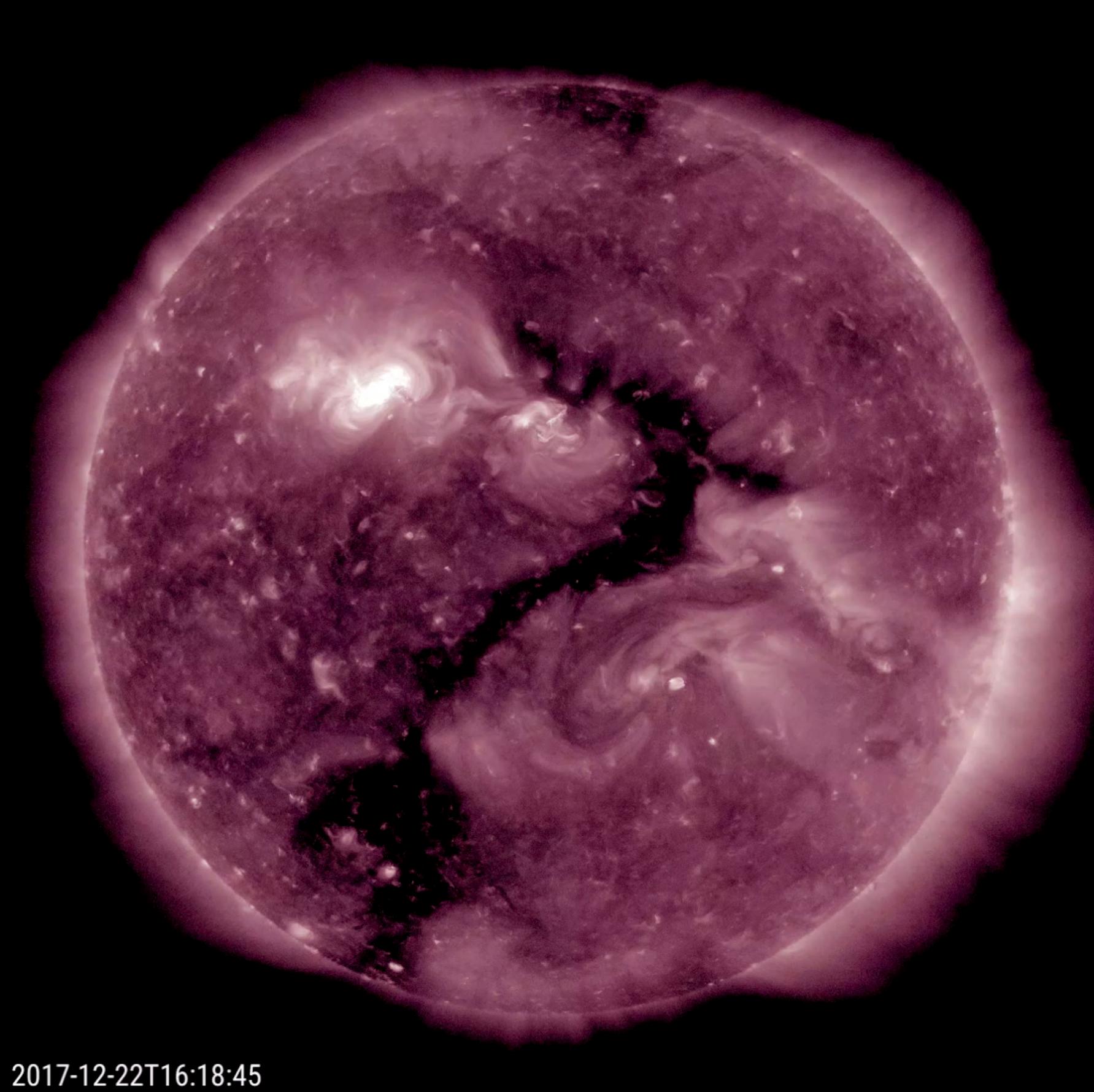
External links
Editor-In-Chief: Henry A Hoff
- Pages with citations using unsupported parameters
- Pages using citations with accessdate and no URL
- CS1 maint: Multiple names: authors list
- CS1 maint: Uses editors parameter
- CS1 errors: ISBN
- Pages with URL errors
- Pages with citations using unnamed parameters
- CS1 maint: Explicit use of et al.
- Pages with broken file links
- Radiation astronomy lectures
- Resources last modified in October 2019